Predicting the likelihood and severity of financial crises over the medium term with a cyclical systemic risk indicator
Published as part of the Financial Stability Review May 2018.
This special feature presents a tractable, transparent and broad-based cyclical systemic risk indicator (CSRI) that captures risks stemming from domestic credit, real estate markets, asset prices, external imbalances and cross-country spillovers. The CSRI increases on average several years before the onset of systemic financial crises and its level is highly correlated with measures of crisis severity. Model estimates suggest that high values of the CSRI contain information about large declines in real GDP growth three to four years down the road, as it precedes shifts in the entire distribution of future real GDP growth and especially of its left tail. Given its timely signals, the CSRI is a useful analytical tool for macroprudential policymakers to complement other existing analytical tools.
1 Introduction
The global financial crisis has shown that the unravelling of systemic risk can have large detrimental effects on the output and welfare of societies. Lo Duca et al. (2017) estimate that output losses during past systemic financial crises in EU countries amounted to 8% of GDP on average, and Laeven and Valencia (2012) estimate that during past banking crises across a large sample of countries worldwide output losses amounted on average to 23% of GDP.[2] In order to prevent systemic financial crises or mitigate their impact in the future, it is therefore essential to have measures of systemic risk that provide sufficient lead time for policymakers to act in a countercyclical manner.
The total credit-to-GDP gap of the Basel III framework (the “Basel gap”)[3] provides a useful starting point for measuring the cyclical dimension of systemic risk. According to the classification in Borio (2003)[4], the cyclical dimension of systemic risk is concerned with the build-up of macro-financial imbalances over time, while the cross-sectional dimension of systemic risk is concerned with the build-up of risk due to the (micro) structure of the financial system. Various studies have shown that the Basel gap is a useful measure of cyclical systemic risk, as it provides good aggregate early warning signals for systemic banking crises.[5]
However, the Basel gap has some shortcomings when it comes to measuring cyclical systemic risk. First, the Basel gap can be biased downward after prolonged credit booms, because the longer the boom period persists the greater will be the portion of the credit excesses contained in the estimate of the trend.[6] Second, the Basel gap is sensitive to the length of the underlying time series, reducing the robustness of the signal for some euro area countries owing to short credit series of 10-15 years. Third, issues of interpretation and communication may arise, as the Basel gap can decrease in situations where the credit-to-GDP ratio increases strongly but does so at a slower pace than the trend component. In view of these shortcomings, there is a need to develop complementary measures of cyclical systemic risk.
This special feature presents a new composite cyclical systemic risk indicator (CSRI) with high predictive power for both the likelihood and the severity of systemic financial crises over the medium term. The CSRI is a tractable, transparent, and broad-based composite indicator that captures risks from developments in domestic credit, real estate markets, asset prices, external imbalances and cross-country spillovers. The indicator increases on average several years before the onset of historical systemic financial crises in euro area countries and its level is highly correlated with measures of crisis severity, such as declines in real GDP. Estimates based on econometric models suggest that high CSRI values contain information about large declines in real GDP growth three to four years down the road and especially about the left tail of the GDP growth distribution.
The remainder of this special feature presents the features and empirical properties of the CSRI in more detail. The CSRI is designed to indicate the build-up of cyclical systemic risk in a timely manner in order to allow preventive macroprudential policy action. It complements the financial stability risk index (FSRI) presented in Special Feature A, which focuses on a much shorter lead time ahead of financial stress by also exploring the information on the cross-sectional dimension of systemic risk contained in financial market prices. Both indicators together thus provide comprehensive model-based information to support the assessment of financial stability risks at any point in time for different prediction horizons.
Box A A generic procedure for constructing a tractable composite systemic risk indicator
This box presents a generic procedure for constructing a broad-based systemic risk indicator that is tractable, transparent, and easily interpretable for policy use. Tractability and transparency are considered to be important characteristics for a composite systemic risk indicator in order to ease interpretation and communication of systemic risk signals. Furthermore, policy action using granular macroprudential instruments requires a means to easily identify the drivers behind risk signals in order to address the specific sources of systemic risks.
The generic procedure has four building blocks and combines methods employed in the early warning literature with a simple and intuitive aggregation method. The four general building blocks are: (i) selection of a set of relevant indicator categories for the risk of interest; (ii) selection of the optimal early warning indicator for each of the indicator categories; (iii) normalisation of each optimal early warning indicator based on the pooled median and standard deviation across countries and time; and (iv) linear aggregation of the normalised early warning indicators into a composite systemic risk indicator based on optimal indicator weights.
Formally, the generic composite systemic risk indicator (SRI) is defined as a weighted average of the normalised sub-indictors:
where represents the normalised sub-indicator, with indicating a country, the time period, and the sub-indicator. represents the relative weight in the composite indicator attributed to the sub-indicator. Pooled indicator normalisation and constant weights across countries and time implicitly assumes that there are common indicator patterns across the crises experienced by individual European countries at different points in time which, once extracted, are useful in identifying the build-up of systemic risk. These risk signals based on common patterns can then be complemented by expert judgement, taking into account country-specificities in a detailed manner.
The weights for aggregating sub-indicators are chosen to optimise the early warning properties of the composite systemic risk indicator. The optimal sub-indicator weights are obtained by running a linear regression of a crisis vulnerability indicator on the normalised sub-indicators and using the estimated coefficients as weights, after constraining them to sum to 1.[7] This regression approach provides the optimal linear combination of the underlying sub-indicators to identify vulnerable periods. Country-specific weights are difficult to estimate, owing to the scarcity of crises at the country level.
The generic procedure for constructing a composite systemic risk indicator can be applied to different sectors of the economy or different systemic risk categories. By varying the crisis episodes of interest and the relevant categories for the early warning indicators, the focus of the early warning assessment can be adjusted. For example, in the context of domestic cyclical systemic risks, relevant indicator categories include credit developments, real estate markets and asset prices. For monitoring systemic risks within the banking sector, indicator categories could include capital adequacy, liquidity and asset quality.
2 A cyclical systemic risk indicator for euro area countries
The new cyclical systemic risk indicator (CSRI) is constructed in a three-step procedure to capture both domestic and cross-country spillover risks. First, a domestic systemic risk indicator (d-SRI) is constructed at the country level to capture the build-up of cyclical imbalances in the domestic non-financial private sector. Second, an exposure-based spillover systemic risk indicator (e-SRI) is constructed to capture a country’s exposure to the build-up of imbalances abroad. Third, the d-SRI and the e-SRI are combined as sub-components of the CSRI. Each of these three steps is discussed in more detail in the following paragraphs.
The design of the d-SRI follows the generic procedure outlined in Box A and covers a broad range of risk categories capturing domestic vulnerabilities. BCBS guidance, the CRD IV and ESRB Recommendation ESRB/2014/1 assign a central role to the credit-to-GDP gap in the measurement of cyclical systemic risks. However, additional risk indicator categories can cover other dimensions of cyclical systemic risks and complement signals from the Basel gap. Therefore, as recommended by the ESRB, the d-SRI considers: (a) measures of potential overvaluation of property prices; (b) measures of credit developments; (c) measures of external imbalances; (d) measures of private sector debt burden; and (e) measures of potential mispricing of risk.[8]
For each of the categories chosen for risk monitoring, the best univariate early warning indicator is identified and included in the d-SRI (see Box B).[9] The six sub-indicators that make up the d-SRI are: (i) the two-year change in the bank credit-to-GDP ratio; (ii) the two-year growth rate of real total credit (CPI-deflated); (iii) the two-year change in the debt service ratio (DSR); (iv) the three-year change in the residential real estate (RRE) price-to-income ratio; (v) the three-year growth rate of real equity prices (CPI-deflated); and (vi) the current account-to-GDP ratio. All of the sub-indicators of the d-SRI are in either two-year or three-year transformations, as these are found to have the best overall early warning properties, i.e. they perform better than shorter-term transformations or HP-filtered gaps.[10]
Box B Selection of useful early warning indicators for signalling systemic financial crises
This box presents the results of a comprehensive evaluation exercise for a large set of early warning indicators using the new ECB/ESRB EU crises database.[11] This new database for financial crises in European countries was developed by the substructures of the ECB’s Financial Stability Committee (FSC) and the ESRB’s Advisory Technical Committee (ATC) with the specific purpose of supporting the calibration of models for macroprudential analysis.
The baseline definition of financial crises encompasses all systemic crises that are not purely imported, as the focus of the evaluation exercise is on the build-up of domestic imbalances. For the early warning exercise, the crises variable is converted into a vulnerability indicator that takes the value 1 during a time window of twelve to five quarters before the start of a crisis and zero otherwise. This window is set to cover up to three years of pre-crisis horizon so as to give policymakers sufficient lead time to take action. The relevant sample for the early warning exercise comprises all euro area countries plus Denmark, Sweden and the United Kingdom and covers the period from the first quarter of 1970 to the fourth quarter of 2016.
Various statistical transformations are tested for a large set of underlying indicators covering credit, real estate, asset prices, debt service, and external imbalances considered relevant for the build-up of cyclical systemic risks. The following transformations are used: one-quarter, one-year, two-year and three-year growth rates and/or changes in ratios to GDP,[12] one-sided HP-filtered gaps with a smoothing parameter of 400,000 and 26,000, and the levels of the variables if deemed relevant. Only indicators that have at least 1,500 country-quarter observations are considered.
The early warning indicators are evaluated on the basis of a combination of their in-sample and out-of-sample signalling performance. The in-sample early warning properties are evaluated with the AUROC[13] for a pre-crisis horizon of twelve to five quarters.[14] The out-of-sample early warning properties are evaluated using the relative usefulness measure[15] based on a recursive quasi real-time exercise starting in the first quarter of 2000 for the same vulnerability indicator and balanced policymaker preferences between missing crises and issuing false alarms.
The main result of the evaluation exercise is that simple transformations of credit and asset price variables can have similar or even better early warning properties than the Basel gap for the set of selected EU countries as a whole (Chart A). For domestically driven systemic financial crises in euro area countries, Denmark, Sweden and the United Kingdom, bank credit indicators tend to have better early warning properties than total credit indicators. Moreover, two or three-year changes in credit-to-GDP ratios tend to have better signalling properties than “gaps” derived using a recursive HP filter. Overall, the two-year change in the bank credit-to-GDP ratio is the best performing univariate early warning indicator for domestic systemic financial crises with an in-sample AUROC of 0.84 and an out-of-sample relative usefulness of 0.38. The two-year change in the debt service ratio (DSR) or three-year change in the residential real estate (RRE) price-to-income ratio have slightly better in-sample and out-of-sample early warning performance than the Basel gap.
Chart A
Simple credit and asset price indicators have similar or even better early warning properties for domestic financial crises in euro area countries than the total credit-to-GDP gap
In-sample and out-of-sample early warning properties of the best univariate indicators and the Basel gap
(left-hand scale: in-sample AUROC; right-hand scale: out-of-sample relative usefulness)

Source: ECB calculations based on the ECB/ESRB EU crises database.Notes: The relevant sample for the early warning performance metrics comprises all euro area countries plus Denmark, Sweden and the United Kingdom for the period from Q1 1970 to Q4 2016. “NFPS” stands for “non-financial private sector”. “AUROC” stands for “area under the receiver operating characteristics curve”, which is a global measure of the early warning performance of an indicator. A perfect indicator has an AUROC of 1 and an uninformative indicator an AUROC of 0.5. The in-sample AUROC is computed for a pre-crisis horizon of 12 to 5 quarters based on all systemic financial crises that are not purely foreign-induced from the new ECB/ESRB EU crises database. The out-of-sample early warning properties are evaluated with the relative usefulness for balanced preferences based on a recursive quasi real-time exercise starting in Q1 2000 for the same pre-crisis horizon of 12 to 5 quarters. “Basel gap” refers to the standardised credit-to-GDP gap, which is obtained as the cyclical component of a recursive HP filter with a smoothing parameter of 400,000 applied to the total credit-to-GDP ratio.
Combining early warning indicators into a composite domestic systemic risk indicator further improves the in-sample and out-of-sample early warning properties. The finding that composite risk indicators improve on the early warning performance of single indicators confirms findings in the literature (see, for example, Detken et al. (2014) and references therein).
The d-SRI is constructed as the optimal weighted average of six well-performing normalised early warning indicators. Indicator normalisation is performed by subtracting the median and dividing by the standard deviation of the pooled indicator distribution across countries and time.[16] Indicator weights are chosen to maximise the early warning performance of the d-SRI for domestically-driven systemic financial crises identified in Lo Duca et al. (2017) with a lead time of 12 to 5 quarters (see Box A for technical details). The optimal weighting procedure for the d-SRI assigns the largest weight to the bank credit-to-GDP change (36%), followed by the current account balance (20%), the RRE price-to-income ratio change (17%), real equity price growth (17%), the DSR change (5%), and real total credit growth (5%).
The units of the d-SRI reflect the weighted average deviation of the sub-indicators from their median in multiples of the standard deviation. Hence, assuming that all sub-indicators display the same level of imbalance, a d-SRI value of +1 can be interpreted as all sub-indicators being one standard deviation above their median value from the pooled historical indicator distribution across euro area countries.
To complement the information from the d-SRI, the e-SRI is designed to capture the direct exposure of a country to the build-up of cyclical systemic risks abroad. To capture this notion of cross-country spillover risks, the e-SRI is constructed as an exposure-based weighted average of the d-SRI across all foreign countries from the point of view of the country of interest. For this purpose, the d-SRI is calculated for 45 countries worldwide. The weights for constructing the e-SRI are country-specific and vary over time based on the direct asset-side exposure of each national banking system to all of the other foreign countries.[17] The e-SRI thus captures the country-specific exposure to the build-up of cyclical systemic risks in foreign countries from across the world.
In a final step, the CSRI is obtained as the optimal weighted average of the d-SRI and the e-SRI. In particular, the optimal weights of the two systemic risk indicators are chosen to maximise the early warning performance of the CSRI for all systemic financial crises identified in Lo Duca et al. (2017), with a lead time of 12 to 5 quarters. The set of crises considered for the CSRI is thus broader than the set of “domestic” crises considered for the d-SRI and includes systemic financial crises that were induced by foreign factors.
3 Information content of the cyclical systemic risk indicator about the likelihood of systemic financial crises
The CSRI displays long cycles across euro area countries and tends to increase well before the onset of systemic financial crises (Charts B.1 and B.2). Since the early 1980s the median CSRI across euro area countries displays three peaks with a marked increase before the global financial crisis and subsequent bust (Chart B.1). Currently, the median CSRI still remains at subdued levels, with a large dispersion across individual euro area countries. An inspection of the evolution of the CSRI across past systemic financial crises shows that the indicator starts to increase on average around five years ahead of a crisis and reaches its peak around four to eight quarters before the onset of a systemic financial crisis (Chart B.2). This pattern illustrates the timely risk signals provided by the CSRI.
The CSRI displays long cycles with three peaks since the early 1980s across euro area countries
Cross-country mean, median and interquartile range of the CSRI over time
(x-axis: time; y-axis: CSRI)
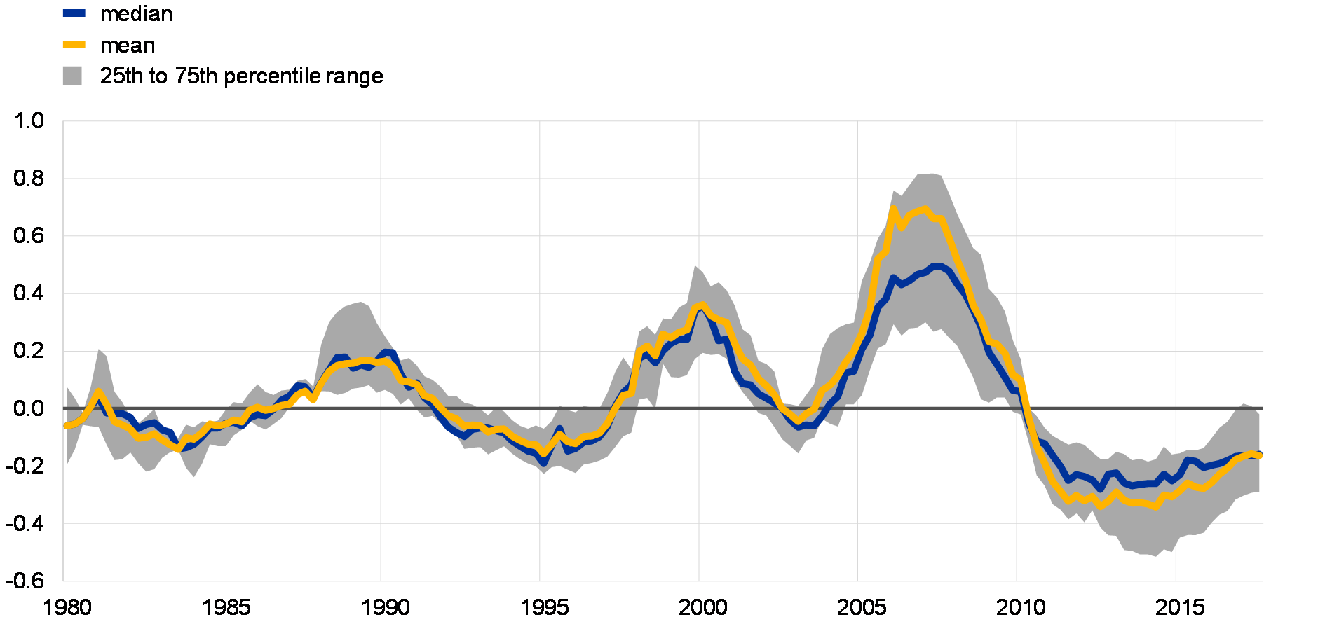
Source: ECB calculations based on various data sources.Notes: The grey shaded area indicates the interquartile range of the CSRI across euro area countries. The CSRI is constructed as a weighted average of the d-SRI and the e-SRI.
The CSRI starts to increase on average around five years before a financial crisis
Cross-country distribution of CSRI values around past systemic financial crises
(x-axis: quarters before/after the start of systemic financial crises; y-axis: CSRI)
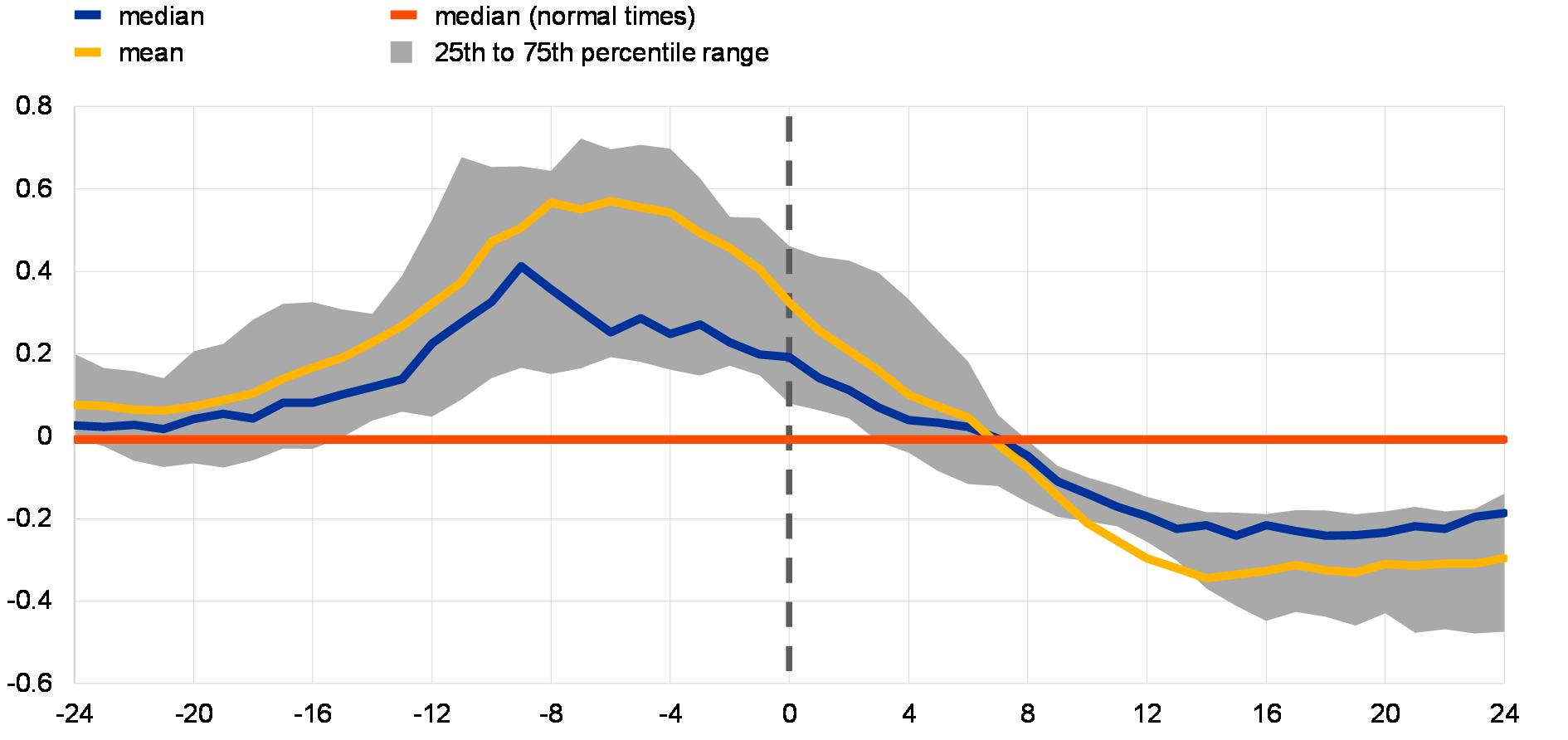
Source: ECB calculations based on various data sources.Notes: The grey shaded area indicates the interquartile range of the CSRI across euro area countries during the 24 quarters before and after systemic financial crises. The orange line indicates the median of the CSRI across euro area countries in “normal times” (not within +/- 6 years of the start of a systemic financial crisis). The dating of systemic financial crises in the chart is based on the ECB/ESRB EU crises database described in Lo Duca et al. (2017).
The early warning properties of the CSRI for systemic financial crises across euro area countries as a whole are superior to those of the credit-to-GDP gap. If one considers all systemic financial crises in the sample, the CSRI attains an AUROC of around 0.85 for a prediction horizon of 12 to 5 quarters, while the total credit-to-GDP gap reaches an AUROC of 0.67.[18] If one considers only domestically-induced systemic financial crises, the d-SRI achieves an AUROC of 0.88 for a prediction horizon of 12 to 5 quarters (see Box B). Moreover, the d-SRI also attains a high out-of-sample relative usefulness of 0.52 based on a quasi-real-time early warning exercise starting in the first quarter of 2000.
The cross-country spillover e-SRI can significantly change the overall cyclical systemic risk assessment for countries with sizeable cross-border exposures (Chart B.3). For example, in the case of Germany, domestic vulnerabilities, as represented by the d-SRI, were subdued ahead of the global financial crisis and would not have indicated heightened cyclical systemic risks. However, risks from foreign spillovers, as measured by the e-SRI, increased considerably between 2003 and 2008, owing to the increasing foreign exposures of the German banking system and the build-up of cyclical systemic risks abroad. A breakdown of the CSRI into the domestic and cross-border spillover components can therefore inform macroprudential policy authorities about the sources of systemic risk.
The domestic and foreign spillover dimensions of cyclical systemic risks provide complementary information, as shown by the example of Germany
CSRI, d-SRI and e-SRI for Germany
(x-axis: time; y-axis: deviation from median)
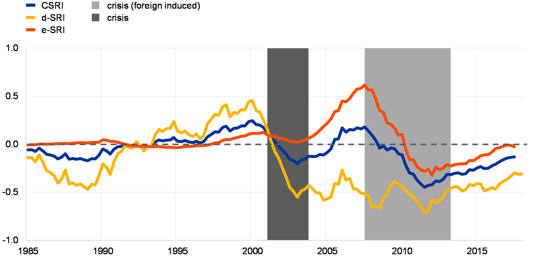
Source: ECB calculations based on various data sources.Notes: The dates of systemic financial crises on the chart are based on the ECB/ESRB EU crises database described in Lo Duca et al. (2017). The dark grey bar indicates a systemic crisis that was due to domestic factors, while the light grey bar indicates a systemic crisis that was induced purely by foreign factors.
The d-SRI can be decomposed into its underlying driving factors, which can help to arrive at a risk narrative and support communication of risk assessments
Decomposition of the d-SRI for the euro area aggregate
(x-axis: date; y-axis: d-SRI and contributions of d-SRI components)
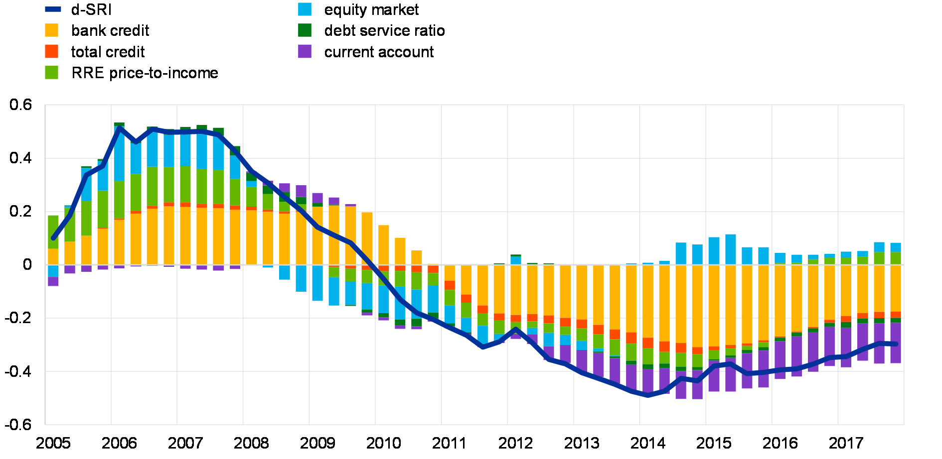
Source: ECB calculations based on various data sources.Notes: The decomposition is based on the d-SRI sub-indicator values in combination with their optimal weights (indicated in brackets): bank credit-to-GDP change (36%), current account balance (20%), RRE price-to-income ratio change (17%), real equity price growth (17%), DSR change (5%), and real total credit growth (5%).
In addition, the tractable nature of the d-SRI allows a straightforward decomposition into driving factors which can help develop an overall risk narrative (Chart B.4). Owing to the weighted linear aggregation of the d-SRI, it can be decomposed into its fundamental driving factors. Such a decomposition can be used to identify whether the domestic cyclical systemic risk build-up is broad-based or driven by selected risk factors and whether individual factors accentuate or attenuate the overall vulnerability. Positive contributions imply that a risk factor is above the cross-country historical median, while negative contributions imply that it is below the median.
4 Information content of the cyclical systemic risk indicator about the severity of systemic financial crises
The level of the d-SRI around the start of past systemic financial crises contains information about the subsequent severity of a crisis. For example, the maximum value of the d-SRI within a six-quarter pre-crisis window displays a high correlation with the subsequent maximum drop in real GDP during systemic financial crises (Chart B.5). Hence, for the 19 domestically-driven systemic financial crises for which d-SRI data are available, large non-financial private sector imbalances, as measured by large values of the d-SRI, have tended to be associated with more severe financial crises, as measured by the maximum output loss.
The level of the d-SRI around the start of past systemic financial crises is highly correlated with output losses that materialised during those crises
Relationship between the d-SRI and drops in real GDP during past systemic financial crises
(x-axis: maximum d-SRI value before a crisis; y-axis: maximum drop in real GDP during a crisis)
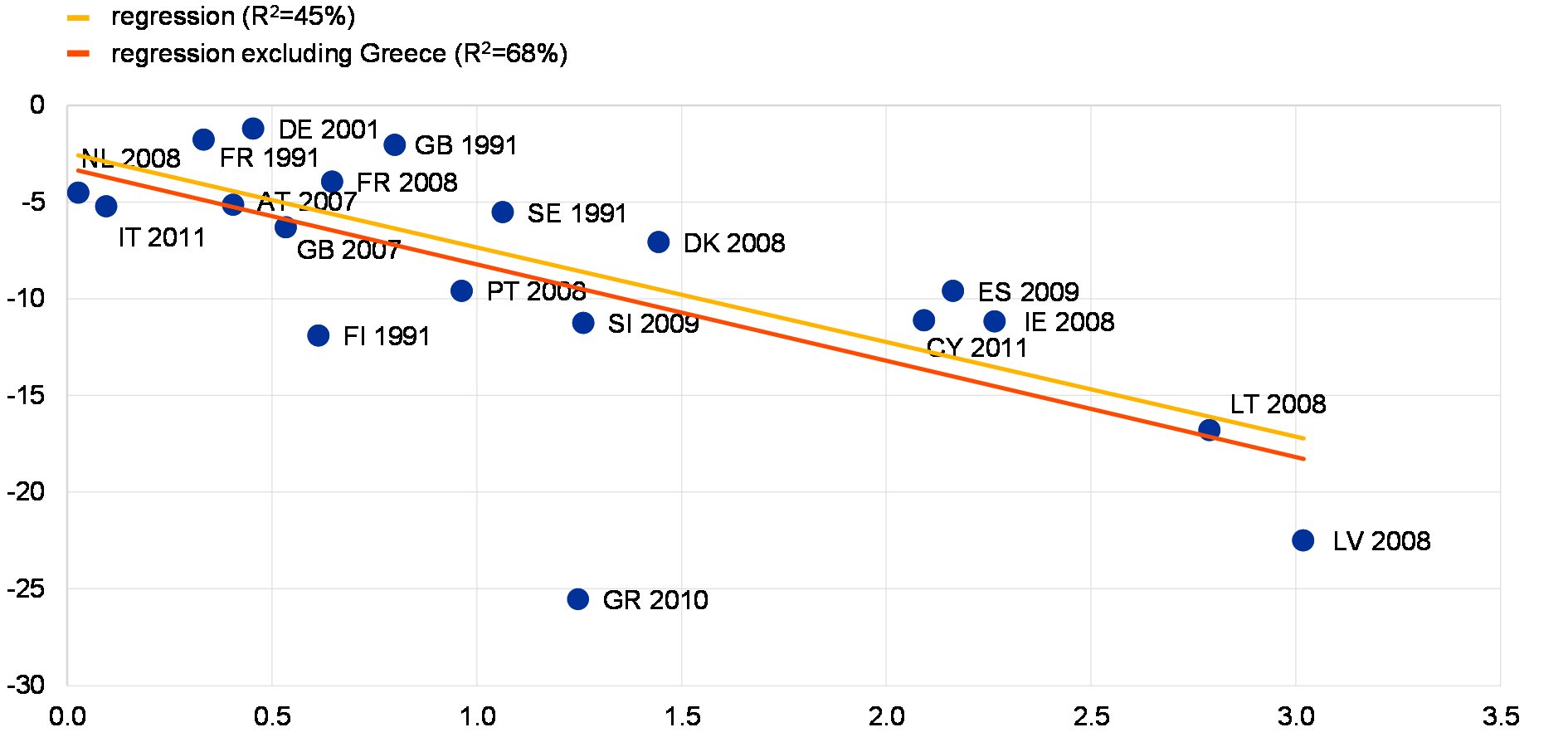
Source: ECB calculations based on various data sources.Notes: The chart shows the peak level of the d-SRI around the start of a systemic financial crisis (defined as six quarters pre-crisis up to the start of a crisis) plotted against the maximum drop in real GDP from peak to trough that materialised during that crisis. The dating of systemic financial crises shown on the chart is based on the new ECB/ESRB EU crises database described in Lo Duca et al. (2017). Purely foreign-induced crises are excluded. In total there are 19 systemic financial crises events in the sample for which d-SRI data are available. Five of these crises materialised before the global financial crisis (FI 1991, FR 1991, GB 1991, SE 1991, DE 2001).
Formal model estimates based on local projections suggest that high values of the CSRI have predictive power for large declines in real GDP growth over the medium term (Chart B.6). For example, across euro area countries, Denmark, Sweden and the United Kingdom, an elevated CSRI value of one standard deviation implies a decline in future real GDP growth of around 4 percentage points three to four years down the road.[19] The predictive power of the CSRI for future GDP growth is statistically significant at the nine quarters ahead horizon and beyond. The strongest predictive power of the CSRI for real GDP growth occurs between 11 and 16 quarters in the future. At shorter horizons it becomes less pronounced, but is still present at the six-years-ahead horizon.
A CSRI value of one standard deviation today leads on average to a decrease in future real GDP growth of around 4 percentage points three years down the road
Local projection impulse response of future real GDP growth to current values of the CSRI
(x-axis: forecast horizon in quarters; y-axis: one-year-ahead real GDP growth rate)
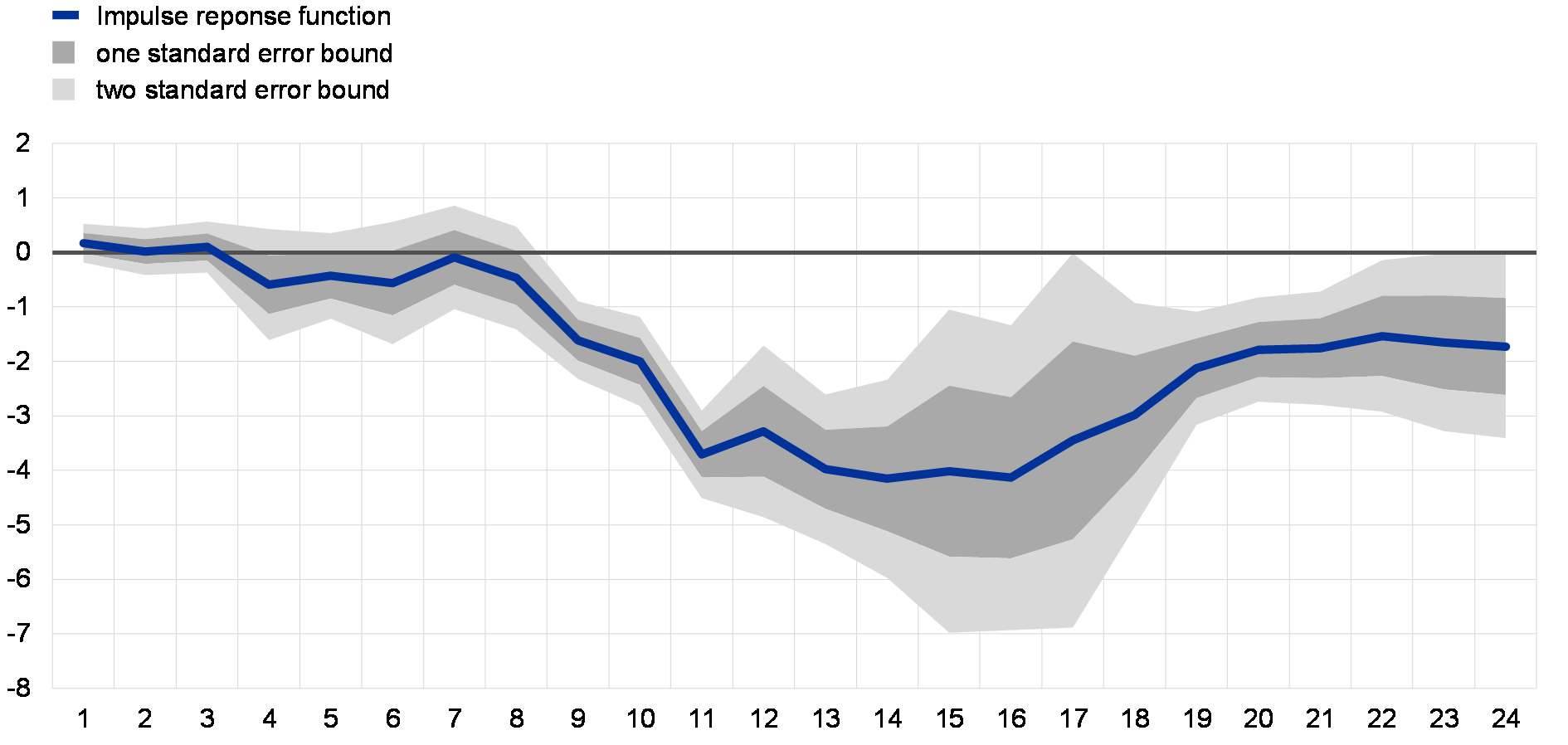
Source: ECB calculations based on various data sources.Notes: The chart displays the impulse response function (IRF) of one-year-ahead real GDP growth to a one standard deviation shock in the CSRI. The IRF is obtained from local projections as proposed by Jordà (2005), controlling for ten lags of one-year-ahead GDP growth rates, ten lags of the CSRI, and country fixed effects. Yellow areas indicate the one and two standard error bounds.
In addition to average real GDP growth, the CSRI has predictive power in particular for the left tail of the growth distribution over the medium term. Quantile impulse responses (Chart B.7) show that the drop in average real GDP growth three to four years ahead shown in chart B.6 is due to a shift of the entire GDP growth distribution, and especially due to a shift in the left tail. For a horizon of 11 to 18 quarters ahead, a one standard deviation value of the CSRI predicts a reduction in the 10th percentile of the real GDP growth distribution by up to 6 percentage points, compared to a range of -2 to -4 percentage points for the 75th and 25th percentiles. Examining quantile loss measures, it is found that the explanatory power of the CSRI for future real GDP growth is strongest for the left tail, proxied by the 10th percentile, and at horizons of 4 to 12 quarters. The foreign CSRI contributes to the explanatory power at horizons of about 12 quarters ahead and beyond.
The CSRI has predictive power for the entire future real GDP growth distribution, and in particular for the left tail of the growth distribution
Quantile regression impulse responses of real GDP growth to current values of the CSRI
(x-axis: forecast horizon in quarters; y-axis: one-year-ahead real GDP growth rate quantile)
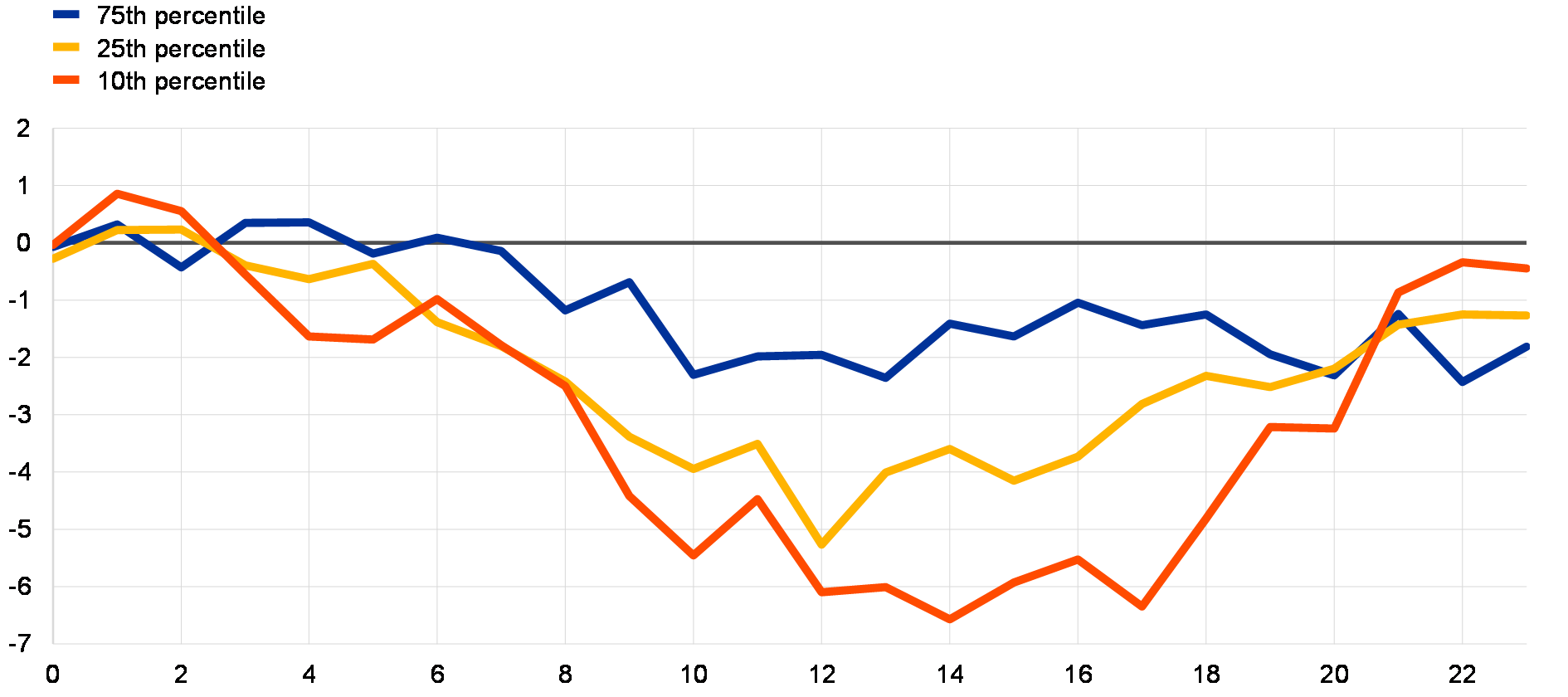
Source: ECB calculations based on various data sources.Notes: The IRF is obtained via local projections based on quantile regressions with ten lags of one-year-ahead GDP growth rates and ten lags of the CSRI.
5 Conclusion
Overall, the CSRI is a tractable and interpretable cyclical systemic risk indicator that contains useful information about the likelihood and severity of systemic financial crises over the medium term. Its main strengths reside in its intuitive decomposition into the macro-financial driving forces of imbalances and in its predictive power for large declines in real GDP growth several years ahead. The CSRI complements the information from other risk signals such as credit-to-GDP gaps, multivariate logit early warning models, financial cycle estimates, semi-structural models of credit excesses, and country-specific indicators. For a detailed systemic risk assessment in the euro area, the CSRI and other formal financial stability indicators will continue to benefit from qualitative information, such as market intelligence. At the same time, refinements are being made to formal systemic risk indicators to raise their predictive performance further, for example by considering variables in levels or country-specific indicator normalisations.
- [1]The analysis and results of this special feature are partly based on Lang, J.H., Izzo, C., Fahr, S. and Ruzicka, J., “Anticipating the bust: A new cyclical systemic risk indicator to assess the likelihood and severity of financial crises”, mimeo, 2018.
- [2]See Lo Duca, M., Koban, A., Basten, M., Bengtsson, E., Klaus, B, Kusmierczyk, P., Lang, J.H., Detken, C. and Peltonen, T., “A new database for financial crises in European countries”, Occasional Paper Series, No 194, ECB, July 2017; and Laeven, L. and Valencia, F., “Systemic Banking Crises Database: An Update”, IMF Working Paper, No WP/12/163, IMF, June 2012.
- [3]The “Basel gap” refers to the total credit-to-GDP gap, which is obtained as the cyclical component from a recursive HP filter with a smoothing parameter of 400,000 applied to the total credit-to-GDP ratio.
- [4]Borio, C., “Towards a macroprudential framework for financial supervision and regulation?”, BIS Working Papers, No 128, BIS, February 2003.
- [5]See for example Borio, C. and Lowe, P., “Asset prices, financial and monetary stability: exploring the nexus”, BIS Working Papers, No 114, July 2002; Borio, C. and Drehmann, M., “Assessing the risk of banking crises – revisited”, BIS Quarterly Review, March 2009; and Aldasoro, I., Borio, C. and Drehmann, M., “Early warning indicators of banking crises: expanding the family”, BIS Quarterly Review, March 2018. See also Detken, C. et al., “Operationalising the countercyclical capital buffer”, Occasional Paper Series, No 5, European Systemic Risk Board (ESRB), June 2014, for EU evidence; and Alessi, L. and Detken, C., “Quasi real time early warning indicators for costly asset price boom/bust cycles”, European Journal of Political Economy, Vol. 27(3), 2011, pp. 520-533, regarding global credit gaps.
- [6]For a detailed exposition of this problem with the Basel gap, see the special feature entitled “Measuring credit gaps for macroprudential policy”, Financial Stability Review, ECB, May 2017.
- [7]The optimal sub-indicator weights are computed by dividing each regression coefficient by the sum of all estimated regression coefficients. This procedure ensures that weights sum to 1. For the application of this generic procedure to the measurement of domestic cyclical systemic risks (i.e. the domestic systemic risk indicator presented in this special feature), a minimum weight for each sub-indicator of 5% is imposed.
- [8]For an overview of risk categories that are recommended to national designated authorities to quantitatively assess cyclical systemic risks, see ESRB Recommendation on guidance for setting countercyclical buffer rates (ESRB/2014/1).
- [9]The exception to this rule is credit: two indicators, one based on bank credit and the other based on total credit, are included in the d-SRI, owing to the prominent role of credit in the context of measuring cyclical systemic risks.
- [10]The use of such simple medium-term transformations for filtering is also supported by the findings in Hamilton, J., “Why you should never use the Hodrick-Prescott filter”, NBER Working Paper, No 23429, 2017, which argues forcefully against using the HP filter.
- [11]See Lo Duca et al. (2017), op. cit.
- [12]All indicators are expressed as annualised averages, e.g. three-year changes are divided by three and two-year changes are divided by two.
- [13]The area under the receiver operating characteristics curve (AUROC) is a global measure of the signalling performance of an early warning indicator. It is computed as the area under the receiver operating characteristics (ROC) curve, which plots the noise ratio (false positive rate) against the signal ratio (true positive rate) for every possible signalling threshold value. An AUROC value of 0.5 indicates an uninformative indicator and a value of 1 indicates a perfect early warning indicator.
- [14]The relative performance of the indicators is robust to considering alternative predictive horizons of sixteen to five quarters based on the benchmark crisis definition from the new ECB/ESRB EU crises database or of twelve to five quarters based on the crisis definition in Detken et al. (2014).
- [15]The relative usefulness measure represents the difference between the loss that a policymaker would get when using the early warning model and the loss when ignoring the model, expressed as a share of the maximum achievable difference. The measure thus gives an idea of how close the early warning model is to a perfect model of crisis prediction for a policymaker with a given preference between type I errors (missing crises) and type II errors (issuing false alarms). See Alessi and Detken (2011), op. cit., regarding usefulness; and Sarlin, P., “On policymakers’ loss functions and the evaluation of early warning systems”, Working Paper Series, No 1509, ECB, 2013, regarding the relative usefulness measure.
- [16]For the current account, the normalised indicator is multiplied by –1 so that higher values indicate more risk. The normalisation based on pooled data moments does not alter the dynamics or the early warning properties of the d-SRI compared to using the raw underlying early warning indicators to compute the d-SRI. The advantage of this normalisation is, however, that the units of the d-SRI have an intuitive interpretation as the weighted average deviation from the historical median, measured in multiples of the historical standard deviation. In addition, owing to the normalisation, the d-SRI weights have a direct interpretation as the contribution of each indicator to the variation of the d-SRI. Robustness exercises show that normalisation with pooled cross-country data moments leads to better quasi-real time early warning performance than normalisation with country-specific data moments.
- [17]This method of taking into account cross-country risk spillovers is based on Lang, J.H., “Cross-Country Linkages and Spill-overs in Early Warning Models for Financial Crises”, mimeo, 2015. Exposure to foreign countries is measured by banking sector total claims vis-à-vis each foreign country and is taken from the BIS locational banking statistics. The foreign exposure measure is expressed as a share of total credit provided to the domestic non-financial private sector. Banking sector asset-side exposure is chosen as a proxy for cross-country financial linkages, given the dominant role of banks in the financial system of most euro area countries.
- [18]Compared to the d-SRI, the AUROC of the CSRI for all crisis events is higher by 0.04. See notes to Chart A in Box B for an explanation of the AUROC concept.
- [19]The estimation is based on local projections as proposed by Jordà, Ò., “Estimation and Inference of Impulse Responses by Local Projections”, American Economic Review, Vol. 95(1), 2005, pp. 161-182, using the sample of euro area countries plus Denmark, Sweden and the United Kingdom between the first quarter of 1970 and the fourth quarter of 2016.


